AWS SageMaker Tutorial: Part 4

Intro

Now we are ready to create a multiple linear regression model using the built in SageMaker algorithms.

Setup

In the setup we need to import our libraries and define the name of our bucket and subfolder for our model

# Boto3 is the Amazon Web Services (AWS) Software Development Kit (SDK) for Python
# Boto3 allows Python developer to write software that makes use of services like Amazon S3 and Amazon EC2

import sagemaker
import boto3
from sagemaker import Session

# Let's create a Sagemaker session
sagemaker_session = sagemaker.Session()
bucket = 'tutorial-sagemaker-insurance-multiple-linear-learner'
prefix = 'multiple_linear_learner' # prefix is the subfolder within the bucket.

# Let's get the execution role for the notebook instance.
# This is the IAM role that you created when you created your notebook instance. You pass the role to the training job.
# Note that AWS Identity and Access Management (IAM) role that Amazon SageMaker can assume to perform tasks on your behalf (for example, reading training results, called model artifacts, from the S3 bucket and writing training results to Amazon S3).
role = sagemaker.get_execution_role()
print(role)

⚠️ The Bucket and Folder that you reference here must already exist, they will not be created for you. If they don't already exist you will get an error later

Convert Data to RecordIO Format

This is the format that is specified in the documentation

import io # The io module allows for dealing with various types of I/O (text I/O, binary I/O and raw I/O).
import numpy as np
import sagemaker.amazon.common as smac # sagemaker common libary

# Code below converts the data in numpy array format to RecordIO format
# This is the format required by Sagemaker Linear Learner

buf = io.BytesIO() # create an in-memory byte array (buf is a buffer I will be writing to)
smac.write_numpy_to_dense_tensor(buf, X_train, y_train.reshape(-1))
buf.seek(0)
# When you write to in-memory byte arrays, it increments 1 every time you write to it
# Let's reset that back to zero

S3 Bucket

Upload Training Data

import os

# Code to upload RecordIO data to S3

# Key refers to the name of the file
key = 'linear-train-data'

# The following code uploads the data in record-io format to S3 bucket to be accessed later for training
boto3.resource('s3').Bucket(bucket).Object(os.path.join(prefix, 'train', key)).upload_fileobj(buf)

# Let's print out the training data location in s3
s3_train_data = 's3://{}/{}/train/{}'.format(bucket, prefix, key)
print('uploaded training data location: {}'.format(s3_train_data))

uploaded training data location: s3://tutorial-sagemaker-insurance-multiple-linear-learner/multiple_linear_learner/train/linear-train-data

Output Artifact Location

# create an output placeholder in S3 bucket to store the linear learner output

output_location = 's3://{}/{}/output'.format(bucket, prefix)
print('Training artifacts will be uploaded to: {}'.format(output_location))

Get Algorithm Container

# This code is used to get the training container of sagemaker built-in algorithms
# all we have to do is to specify the name of the algorithm, that we want to use

# Let's obtain a reference to the linearLearner container image
# Note that all regression models are named estimators
# You don't have to specify (hardcode) the region, get_image_uri will get the current region name using boto3.Session

region = boto3.Session().region_name
container = sagemaker.image_uris.retrieve('linear-learner',region)
container

'382416733822.dkr.ecr.us-east-1.amazonaws.com/linear-learner:1'

Train the Model

# We have pass in the container, the type of instance that we would like to use for training
# output path and sagemaker session into the Estimator.
# We can also specify how many instances we would like to use for training

linear = sagemaker.estimator.Estimator(container,
                                       role,
                                       instance_count = 1,
                                       instance_type = 'ml.c4.xlarge',
                                       output_path = output_location,
                                       sagemaker_session = sagemaker_session,
                                       # reduce cost with spot instances
                                       use_spot_instances = True,
                                       max_run = 300,
                                       max_wait = 600
                                      )


# We can tune parameters like the number of features that we are passing in, type of predictor like 'regressor' or 'classifier', mini batch size, epochs
# Train 32 different versions of the model and will get the best out of them (built-in parameters optimization!)

linear.set_hyperparameters(feature_dim = 8,
                           predictor_type = 'regressor',
                           mini_batch_size = 100,
                           epochs = 100,
                           num_models = 32,
                           loss = 'absolute_loss')

# Now we are ready to pass in the training data from S3 to train the linear learner model

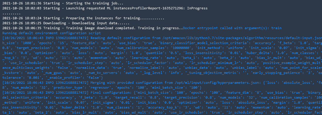
linear.fit({'train': s3_train_data})

# Let's see the progress using cloudwatch logs

This took significantly longer than the previous linear learner model to process

[10/26/2021 18:06:50 INFO 139621688817472] #throughput_metric: host=algo-1, train throughput=4583.929433778798 records/second
[10/26/2021 18:06:50 WARNING 139621688817472] wait_for_all_workers will not sync workers since the kv store is not running distributed
[10/26/2021 18:06:50 WARNING 139621688817472] wait_for_all_workers will not sync workers since the kv store is not running distributed
[2021-10-26 18:06:50.454] [tensorio] [info] epoch_stats={"data_pipeline": "/opt/ml/input/data/train", "epoch": 52, "duration": 0, "num_examples": 1, "num_bytes": 7600}
[2021-10-26 18:06:50.470] [tensorio] [info] epoch_stats={"data_pipeline": "/opt/ml/input/data/train", "epoch": 54, "duration": 14, "num_examples": 11, "num_bytes": 81320}
[10/26/2021 18:06:50 INFO 139621688817472] #train_score (algo-1) : ('absolute_loss_objective', 0.30221866892877025)
[10/26/2021 18:06:50 INFO 139621688817472] #train_score (algo-1) : ('mse', 0.2992234559816735)
[10/26/2021 18:06:50 INFO 139621688817472] #train_score (algo-1) : ('absolute_loss', 0.30221866892877025)
[10/26/2021 18:06:50 INFO 139621688817472] #quality_metric: host=algo-1, train absolute_loss_objective <loss>=0.30221866892877025
[10/26/2021 18:06:50 INFO 139621688817472] #quality_metric: host=algo-1, train mse <loss>=0.2992234559816735
[10/26/2021 18:06:50 INFO 139621688817472] #quality_metric: host=algo-1, train absolute_loss <loss>=0.30221866892877025
[10/26/2021 18:06:50 INFO 139621688817472] Best model found for hyperparameters: {"optimizer": "adam", "learning_rate": 0.1, "wd": 0.01, "l1": 0.0, "lr_scheduler_step": 100, "lr_scheduler_factor": 0.99, "lr_scheduler_minimum_lr": 1e-05}

2021-10-26 18:30:14 Uploading - Uploading generated training model
2021-10-26 18:30:14 Completed - Training job completed
Training seconds: 72
Billable seconds: 30
Managed Spot Training savings: 58.3%

Deploy The Model

# Deploying the model to perform inference

linear_regressor = linear.deploy(initial_instance_count = 1,
                                          instance_type = 'ml.m4.xlarge')

Test The Model

Select Serializers

Now we can pass in our X_test data, but first we must choose which serializer and deserializer we would like to use to transform our data. The documentation states that the incoming data must be in CSV format, so will use the CSV serializer, and then we can pick how we would like to receive the data back. Here we would like it back in JSON format.

from sagemaker.serializers import CSVSerializer
from sagemaker.deserializers import JSONDeserializer

# Content type overrides the data that will be passed to the deployed model, since the deployed model expects data in text/csv format.

# Serializer accepts a single argument, the input data, and returns a sequence of bytes in the specified content type

# Deserializer accepts two arguments, the result data and the response content type, and return a sequence of bytes in the specified content type.

linear_regressor.serializer = CSVSerializer()
linear_regressor.deserializer = JSONDeserializer()

Pass Test Data into Model

and now we can pass our test data into our deployed model

# making prediction on the test data

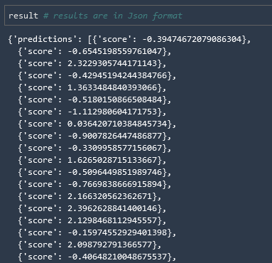
result = linear_regressor.predict(X_test)

and we can see that we have results, but they are scaled and in a JSON object

Shape Results

Let's first convert the data in the object into an array, and then we can scale it back.

# Since the result is in json format, we access the scores by iterating through the scores in the predictions

predictions = np.array([r['score'] for r in result['predictions']])

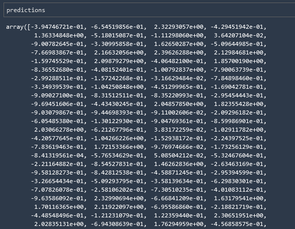
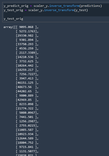
and now we can return the predictions to their original scale

y_predict_orig = scaler_y.inverse_transform(predictions)
y_test_orig = scaler_y.inverse_transform(y_test)

y_test_orig

Review Metrics

Let's review our metrics to see how our model did!

from sklearn.metrics import r2_score, mean_squared_error, mean_absolute_error
from math import sqrt

RMSE = float(format(np.sqrt(mean_squared_error(y_test_orig, y_predict_orig)),'.3f'))
MSE = mean_squared_error(y_test_orig, y_predict_orig)
MAE = mean_absolute_error(y_test_orig, y_predict_orig)
r2 = r2_score(y_test_orig, y_predict_orig)
adj_r2 = 1-(1-r2)*(n-1)/(n-k-1)

print('RMSE =',RMSE, '\nMSE =',MSE, '\nMAE =',MAE, '\nR2 =', r2, '\nAdjusted R2 =', adj_r2) 

RMSE = 6166.98 
MSE = 38031640.86666906 
MAE = 3418.82080646875 
R2 = 0.7550276878607206 
Adjusted R2 = 0.7474609755166501

Delete endpoint

And now let us shut down the endpoint so that we aren't running an EC2 instance for nothing.

# Delete the end-point

linear_regressor.delete_endpoint()

Comments

Recent Work

Basalt

basalt.software

Free desktop AI Chat client, designed for developers and businesses. Unlocks advanced model settings only available in the API. Includes quality of life features like custom syntax highlighting.

Learn More

BidBear

bidbear.io

Bidbear is a report automation tool. It downloads Amazon Seller and Advertising reports, daily, to a private database. It then merges and formats the data into beautiful, on demand, exportable performance reports.

Learn More