AWS SageMaker Tutorial: Part 5
Intro
In this post we will use SageMaker to create a neural network with the goal of predicting health insurance costs. The inputs of our model are:
- Age
- Gender
- BMI
- Number of Children
- Smoking Habit
- Location (Region)
Data Source: Kaggle: Insurance
Dependencies
!pip install tensorflow
import tensorflow as tf
from tensorflow import keras
from tensorflow.keras.layers import Dense, Activation, Dropout, BatchNormalization
from tensorflow.keras.optimizers import Adam
Keras is a deep learning API written in Python, running on top of the machine learning platform TensorFlow. It was developed with a focus on enabling fast experimentation. Being able to go from idea to result as fast as possible is key to doing good research.
Define Network Stack
# optimizer = Adam()
ANN_model = keras.Sequential()
ANN_model.add(Dense(50, input_dim = 8))
ANN_model.add(Activation('relu'))
ANN_model.add(Dense(150))
ANN_model.add(Activation('relu'))
ANN_model.add(Dropout(0.5))
ANN_model.add(Dense(150))
ANN_model.add(Activation('relu'))
ANN_model.add(Dropout(0.5))
ANN_model.add(Dense(50))
ANN_model.add(Activation('linear'))
ANN_model.add(Dense(1))
ANN_model.compile(loss = 'mse', optimizer = 'adam')
ANN_model.summary()
Model: "sequential"
_________________________________________________________________
Layer (type)                 Output Shape              Param #
=================================================================
dense (Dense)                (None, 50)                450
_________________________________________________________________
activation (Activation)      (None, 50)                0
_________________________________________________________________
dense_1 (Dense)              (None, 150)               7650
_________________________________________________________________
activation_1 (Activation)    (None, 150)               0
_________________________________________________________________
dropout (Dropout)            (None, 150)               0
_________________________________________________________________
dense_2 (Dense)              (None, 150)               22650
_________________________________________________________________
activation_2 (Activation)    (None, 150)               0
_________________________________________________________________
dropout_1 (Dropout)          (None, 150)               0
_________________________________________________________________
dense_3 (Dense)              (None, 50)                7550
_________________________________________________________________
activation_3 (Activation)    (None, 50)                0
_________________________________________________________________
dense_4 (Dense)              (None, 1)                 51
=================================================================
Total params: 38,351
Trainable params: 38,351
Non-trainable params: 0
_________________________________________________________________
Run the Model
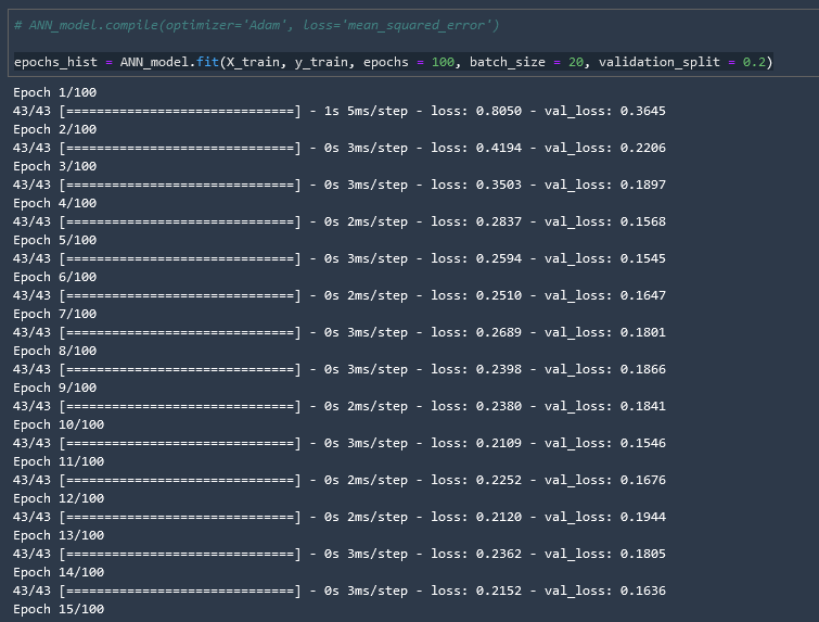
epochs_hist = ANN_model.fit(X_train, y_train, epochs = 100, batch_size = 20, validation_split = 0.2)
result = ANN_model.evaluate(X_test, y_test)
accuracy_ANN = 1 - result
print("Accuracy : {}".format(accuracy_ANN))
9/9 [==============================] - 0s 1ms/step - loss: 0.1649
Accuracy : 0.835088387131691
epochs_hist.history.keys()
dict_keys(['loss', 'val_loss'])
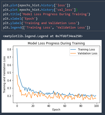
plt.plot(epochs_hist.history['loss'])
plt.plot(epochs_hist.history['val_loss'])
plt.title('Model Loss Progress During Training')
plt.xlabel('Epoch')
plt.ylabel('Training and Validation Loss')
plt.legend(['Training Loss', 'Validation Loss'])
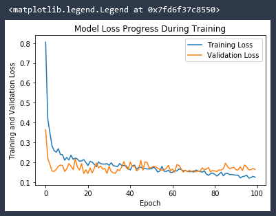
Ideally we would like our validation loss to be on a downward curve along with our Training loss. A flat validation loss trend line, or even upward validation loss trend line, can indicate model saturation. This is when the line is overly fit to the training data, as opposed to being a good general model. The model has become TOO fit. Increasing the density of the model or the number of epochs in this case will give the model a better specific fit to the training data, but could in fact make a it a worse general fit.
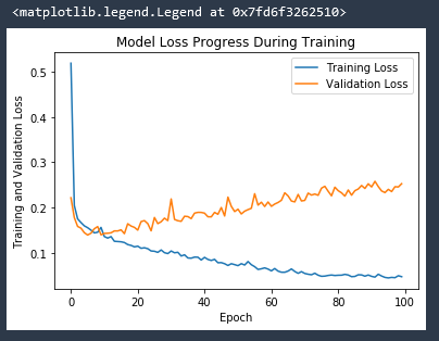
For example if we reduce the number of epochs in our network layers to 50...
ANN_model = keras.Sequential()
ANN_model.add(Dense(50, input_dim = 8))
ANN_model.add(Activation('relu'))
ANN_model.add(Dense(50))
ANN_model.add(Activation('relu'))
ANN_model.add(Dropout(0.5))
ANN_model.add(Dense(50))
ANN_model.add(Activation('relu'))
ANN_model.add(Dropout(0.5))
ANN_model.add(Dense(50))
ANN_model.add(Activation('linear'))
ANN_model.add(Dense(1))
ANN_model.compile(loss = 'mse', optimizer = 'adam')
ANN_model.summary()
We can see that our validation loss is actually much more closely fit to our training loss!
And if we remove the Dropout layers from the network our validation loss explodes!
Predictions vs True Values
If predictions and true values were 100% matching they would both lie on a perfect 45 degree line
y_predict = ANN_model.predict(X_test)
plt.plot(y_test, y_predict, "^", color = 'r')
plt.xlabel('Model Predictions')
plt.ylabel('True Values')
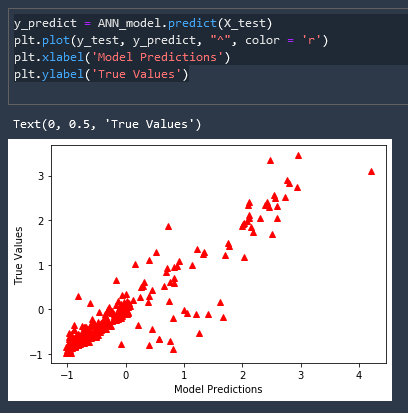
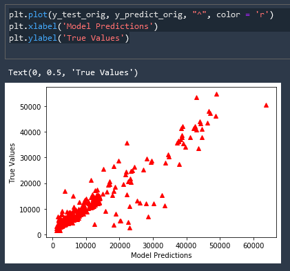
This is great but our labels and scale are nonsensical, let us inverse the scaling of this data and add meaningful labels
y_predict_orig = scaler_y.inverse_transform(y_predict)
y_test_orig = scaler_y.inverse_transform(y_test)

plt.plot(y_test_orig, y_predict_orig, "^", color = 'r')
plt.xlabel('Model Predictions')
plt.ylabel('True Values')
Error Metrics
k = X_test.shape[1]
n = len(X_test)
n

from sklearn.metrics import r2_score, mean_squared_error, mean_absolute_error
from math import sqrt

RMSE = float(format(np.sqrt(mean_squared_error(y_test_orig, y_predict_orig)),'.3f'))
MSE = mean_squared_error(y_test_orig, y_predict_orig)
MAE = mean_absolute_error(y_test_orig, y_predict_orig)
r2 = r2_score(y_test_orig, y_predict_orig)
adj_r2 = 1-(1-r2)*(n-1)/(n-k-1)

print('RMSE =',RMSE, '\nMSE =',MSE, '\nMAE =',MAE, '\nR2 =', r2, '\nAdjusted R2 =', adj_r2)
RMSE = 4878.759
MSE = 23802292.0
MAE = 2834.1655
R2 = 0.8466828566272102
Adjusted R2 = 0.8419471919670468
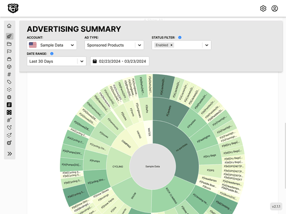
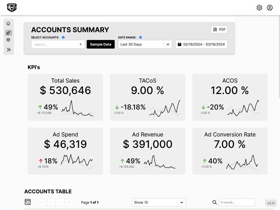
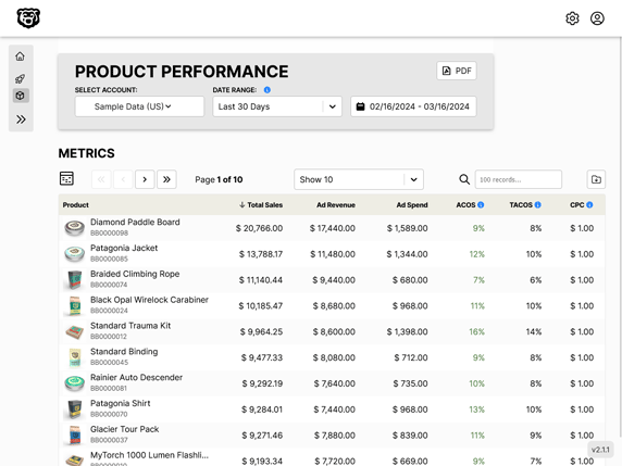
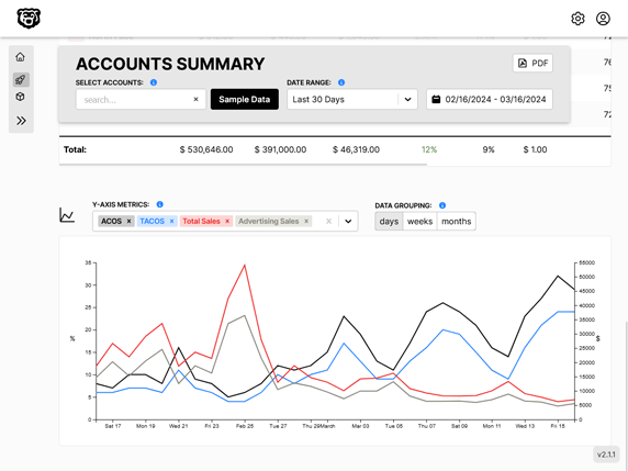
Automated Amazon Reports
Automatically download Amazon Seller and Advertising reports to a private database. View beautiful, on demand, exportable performance reports.