AWS SageMaker Tutorial: Part 6
Intro
In this tutorial we will forecast sales based on historical data.
The dataset contains weekly sales from 99 departments belonging to 45 different stores.
The data contains holidays and promotional markdowns offered by various stores and several departments throughout the year.
The data consists of three sheets:
- Stores
- Features
- Sales
This model will use a high order polynomial regression (complex)
Import Libraries
import pandas as pd
import numpy as np
import seaborn as sns
import matplotlib.pyplot as plt
import zipfile
Import Datasets
# import the csv files using pandas
features = pd.read_csv('Features_data_set.csv')
sales = pd.read_csv('sales_data_set.csv')
stores = pd.read_csv('stores_data_set.csv')
Shape Data
Using the methods we have noted in Ncoughlin: Python Data Manipulation
We have merged our three csv files into one datafield assigned the value df. And merged a new column onto the end of the data called Month which we extracted from the date column with a get_month function.
# defining a function get_month which takes a datetime as an argument
def get_month(datetime):
    # and returns the second string split as an integer
    return int(str(datetime).split('-')[1])
and we can see an example of that working here
get_month('2020-12-31')
12
And we can then apply that function to our datafield df targeting the ['Date'] column
df['Month'] = df['Date'].apply(get_month)
We have also converted the IsHoliday boolean to float32 numeric values (1/0), and also extracted the month from the date and put it in it's own column at the end. That gives us the current shape (random sample of ten rows).
| Store | Dept | Date | Weekly_Sales | IsHoliday | Temperature | Fuel_Price | MarkDown1 | MarkDown2 | MarkDown3 | MarkDown4 | MarkDown5 | CPI | Unemployment | Type | Size | Month | |
|---|---|---|---|---|---|---|---|---|---|---|---|---|---|---|---|---|---|
| 263805 | 27 | 58 | 2011-12-23 00:00:00 | 230 | 0 | 41.59 | 3.587 | 2415.4 | 239.89 | 1438.33 | 209.34 | 2976.85 | 140.529 | 7.906 | A | 204184 | 12 |
| 125050 | 13 | 36 | 2012-01-13 00:00:00 | 580.73 | 0 | 25.61 | 3.056 | 3627.07 | 14887.9 | 119.93 | 798.48 | 4668.82 | 130.244 | 6.104 | A | 219622 | 1 |
| 234570 | 24 | 59 | 2012-02-24 00:00:00 | 366.67 | 0 | 37.35 | 3.917 | 10065.8 | 10556.7 | 2.2 | 6791.1 | 9440.12 | 137.341 | 8.659 | A | 203819 | 2 |
| 234986 | 24 | 37 | 2012-06-04 00:00:00 | 3240.93 | 0 | 45.25 | 4.143 | 24195 | 0 | 59.68 | 3082.34 | 5170.39 | 137.797 | 8.983 | A | 203819 | 6 |
| 341029 | 36 | 82 | 2010-11-06 00:00:00 | 3847.78 | 0 | 82.3 | 2.615 | 0 | 0 | 0 | 0 | 0 | 210.214 | 8.464 | A | 39910 | 11 |
| 101838 | 11 | 32 | 2011-11-03 00:00:00 | 7377.45 | 0 | 63.29 | 3.459 | 0 | 0 | 0 | 0 | 0 | 217.465 | 7.551 | A | 207499 | 11 |
| 347652 | 37 | 46 | 2010-07-16 00:00:00 | 8194.4 | 0 | 84.43 | 2.623 | 0 | 0 | 0 | 0 | 0 | 209.863 | 8.36 | C | 39910 | 7 |
| 384018 | 41 | 71 | 2010-03-12 00:00:00 | 3411.52 | 0 | 33 | 2.712 | 0 | 0 | 0 | 0 | 0 | 190.993 | 7.508 | A | 196321 | 3 |
| 185430 | 19 | 8 | 2012-04-27 00:00:00 | 42555.6 | 0 | 42.45 | 4.163 | 3735.3 | -265.76 | 52.82 | 67.72 | 2959.27 | 137.978 | 8.15 | A | 203819 | 4 |
| 89006 | 10 | 11 | 2010-06-25 00:00:00 | 38635.2 | 0 | 90.32 | 3.084 | 0 | 0 | 0 | 0 | 0 | 126.127 | 9.524 | B | 126512 | 6 |
Next we can drop the date column because we only really want to predict sales by month and we have extracted the month already
# Drop the date
df_target = df['Weekly_Sales']
df_final = df.drop(columns = ['Weekly_Sales', 'Date'])
Lastly we still have a couple of columns that we need to break out into unique values with dummies so that we can group them later in the analysis. Namely Type, Store and Dept. Therefore we use the get_dummies() method.
df_final = pd.get_dummies(df_final, columns = ['Type', 'Store', 'Dept'], drop_first = True)
Which now gives us a very large number of columns
df_final.shape
(421570, 137)
And we can see that every Type, Store and Dept has it's own column now.
| IsHoliday | Temperature | Fuel_Price | MarkDown1 | MarkDown2 | MarkDown3 | MarkDown4 | MarkDown5 | CPI | Unemployment | Size | Month | Type_B | Type_C | Store_2 | Store_3 | Store_4 | Store_5 | Store_6 | Store_7 | Store_8 | Store_9 | Store_10 | Store_11 | Store_12 | Store_13 | Store_14 | Store_15 | Store_16 | Store_17 | Store_18 | Store_19 | Store_20 | Store_21 | Store_22 | Store_23 | Store_24 | Store_25 | Store_26 | Store_27 | Store_28 | Store_29 | Store_30 | Store_31 | Store_32 | Store_33 | Store_34 | Store_35 | Store_36 | Store_37 | Store_38 | Store_39 | Store_40 | Store_41 | Store_42 | Store_43 | Store_44 | Store_45 | Dept_2 | Dept_3 | Dept_4 | Dept_5 | Dept_6 | Dept_7 | Dept_8 | Dept_9 | Dept_10 | Dept_11 | Dept_12 | Dept_13 | Dept_14 | Dept_16 | Dept_17 | Dept_18 | Dept_19 | Dept_20 | Dept_21 | Dept_22 | Dept_23 | Dept_24 | Dept_25 | Dept_26 | Dept_27 | Dept_28 | Dept_29 | Dept_30 | Dept_31 | Dept_32 | Dept_33 | Dept_34 | Dept_35 | Dept_36 | Dept_37 | Dept_38 | Dept_39 | Dept_40 | Dept_41 | Dept_42 | Dept_43 | Dept_44 | Dept_45 | Dept_46 | Dept_47 | Dept_48 | Dept_49 | Dept_50 | Dept_51 | Dept_52 | Dept_54 | Dept_55 | Dept_56 | Dept_58 | Dept_59 | Dept_60 | Dept_65 | Dept_67 | Dept_71 | Dept_72 | Dept_74 | Dept_77 | Dept_78 | Dept_79 | Dept_80 | Dept_81 | Dept_82 | Dept_83 | Dept_85 | Dept_87 | Dept_90 | Dept_91 | Dept_92 | Dept_93 | Dept_94 | Dept_95 | Dept_96 | Dept_97 | Dept_98 | Dept_99 | |
|---|---|---|---|---|---|---|---|---|---|---|---|---|---|---|---|---|---|---|---|---|---|---|---|---|---|---|---|---|---|---|---|---|---|---|---|---|---|---|---|---|---|---|---|---|---|---|---|---|---|---|---|---|---|---|---|---|---|---|---|---|---|---|---|---|---|---|---|---|---|---|---|---|---|---|---|---|---|---|---|---|---|---|---|---|---|---|---|---|---|---|---|---|---|---|---|---|---|---|---|---|---|---|---|---|---|---|---|---|---|---|---|---|---|---|---|---|---|---|---|---|---|---|---|---|---|---|---|---|---|---|---|---|---|---|---|---|---|---|
| 124330 | 0 | 43.51 | 3.538 | 0 | 0 | 0 | 0 | 0 | 129.805 | 6.392 | 219622 | 4 | 0 | 0 | 0 | 0 | 0 | 0 | 0 | 0 | 0 | 0 | 0 | 0 | 0 | 1 | 0 | 0 | 0 | 0 | 0 | 0 | 0 | 0 | 0 | 0 | 0 | 0 | 0 | 0 | 0 | 0 | 0 | 0 | 0 | 0 | 0 | 0 | 0 | 0 | 0 | 0 | 0 | 0 | 0 | 0 | 0 | 0 | 0 | 0 | 0 | 0 | 0 | 0 | 0 | 0 | 0 | 0 | 0 | 0 | 0 | 0 | 0 | 0 | 0 | 0 | 0 | 0 | 0 | 0 | 0 | 0 | 0 | 0 | 0 | 0 | 0 | 0 | 0 | 0 | 0 | 0 | 0 | 0 | 0 | 0 | 0 | 0 | 0 | 0 | 0 | 0 | 0 | 0 | 0 | 0 | 0 | 0 | 0 | 0 | 0 | 0 | 0 | 1 | 0 | 0 | 0 | 0 | 0 | 0 | 0 | 0 | 0 | 0 | 0 | 0 | 0 | 0 | 0 | 0 | 0 | 0 | 0 | 0 | 0 | 0 | 0 | 0 |
| 31488 | 0 | 78.08 | 2.698 | 0 | 0 | 0 | 0 | 0 | 126.064 | 7.372 | 205863 | 8 | 0 | 0 | 0 | 0 | 1 | 0 | 0 | 0 | 0 | 0 | 0 | 0 | 0 | 0 | 0 | 0 | 0 | 0 | 0 | 0 | 0 | 0 | 0 | 0 | 0 | 0 | 0 | 0 | 0 | 0 | 0 | 0 | 0 | 0 | 0 | 0 | 0 | 0 | 0 | 0 | 0 | 0 | 0 | 0 | 0 | 0 | 0 | 0 | 0 | 0 | 0 | 0 | 0 | 0 | 0 | 0 | 0 | 0 | 0 | 0 | 0 | 0 | 0 | 0 | 0 | 0 | 0 | 0 | 1 | 0 | 0 | 0 | 0 | 0 | 0 | 0 | 0 | 0 | 0 | 0 | 0 | 0 | 0 | 0 | 0 | 0 | 0 | 0 | 0 | 0 | 0 | 0 | 0 | 0 | 0 | 0 | 0 | 0 | 0 | 0 | 0 | 0 | 0 | 0 | 0 | 0 | 0 | 0 | 0 | 0 | 0 | 0 | 0 | 0 | 0 | 0 | 0 | 0 | 0 | 0 | 0 | 0 | 0 | 0 | 0 | 0 |
| 248023 | 0 | 61.65 | 2.906 | 0 | 0 | 0 | 0 | 0 | 132.294 | 8.512 | 152513 | 5 | 0 | 0 | 0 | 0 | 0 | 0 | 0 | 0 | 0 | 0 | 0 | 0 | 0 | 0 | 0 | 0 | 0 | 0 | 0 | 0 | 0 | 0 | 0 | 0 | 0 | 0 | 1 | 0 | 0 | 0 | 0 | 0 | 0 | 0 | 0 | 0 | 0 | 0 | 0 | 0 | 0 | 0 | 0 | 0 | 0 | 0 | 0 | 0 | 0 | 0 | 0 | 0 | 0 | 0 | 0 | 0 | 0 | 0 | 0 | 0 | 0 | 0 | 1 | 0 | 0 | 0 | 0 | 0 | 0 | 0 | 0 | 0 | 0 | 0 | 0 | 0 | 0 | 0 | 0 | 0 | 0 | 0 | 0 | 0 | 0 | 0 | 0 | 0 | 0 | 0 | 0 | 0 | 0 | 0 | 0 | 0 | 0 | 0 | 0 | 0 | 0 | 0 | 0 | 0 | 0 | 0 | 0 | 0 | 0 | 0 | 0 | 0 | 0 | 0 | 0 | 0 | 0 | 0 | 0 | 0 | 0 | 0 | 0 | 0 | 0 | 0 |
| 83718 | 0 | 89.33 | 3.533 | 0 | 0 | 0 | 0 | 0 | 219.382 | 6.404 | 125833 | 2 | 1 | 0 | 0 | 0 | 0 | 0 | 0 | 0 | 0 | 1 | 0 | 0 | 0 | 0 | 0 | 0 | 0 | 0 | 0 | 0 | 0 | 0 | 0 | 0 | 0 | 0 | 0 | 0 | 0 | 0 | 0 | 0 | 0 | 0 | 0 | 0 | 0 | 0 | 0 | 0 | 0 | 0 | 0 | 0 | 0 | 0 | 0 | 0 | 0 | 0 | 0 | 0 | 0 | 0 | 0 | 0 | 0 | 0 | 0 | 0 | 0 | 0 | 0 | 0 | 0 | 0 | 0 | 0 | 0 | 0 | 0 | 0 | 0 | 0 | 0 | 0 | 0 | 0 | 0 | 0 | 0 | 0 | 0 | 0 | 0 | 0 | 0 | 1 | 0 | 0 | 0 | 0 | 0 | 0 | 0 | 0 | 0 | 0 | 0 | 0 | 0 | 0 | 0 | 0 | 0 | 0 | 0 | 0 | 0 | 0 | 0 | 0 | 0 | 0 | 0 | 0 | 0 | 0 | 0 | 0 | 0 | 0 | 0 | 0 | 0 | 0 |
| 27729 | 0 | 72.83 | 3.891 | 5359.22 | 1673.42 | 3 | 682.03 | 1371.55 | 225.014 | 6.664 | 37392 | 4 | 1 | 0 | 0 | 1 | 0 | 0 | 0 | 0 | 0 | 0 | 0 | 0 | 0 | 0 | 0 | 0 | 0 | 0 | 0 | 0 | 0 | 0 | 0 | 0 | 0 | 0 | 0 | 0 | 0 | 0 | 0 | 0 | 0 | 0 | 0 | 0 | 0 | 0 | 0 | 0 | 0 | 0 | 0 | 0 | 0 | 0 | 0 | 0 | 0 | 0 | 0 | 0 | 0 | 0 | 0 | 0 | 0 | 0 | 0 | 0 | 0 | 0 | 0 | 0 | 0 | 0 | 0 | 0 | 0 | 0 | 0 | 0 | 0 | 0 | 0 | 0 | 0 | 0 | 0 | 0 | 0 | 0 | 0 | 0 | 0 | 0 | 0 | 1 | 0 | 0 | 0 | 0 | 0 | 0 | 0 | 0 | 0 | 0 | 0 | 0 | 0 | 0 | 0 | 0 | 0 | 0 | 0 | 0 | 0 | 0 | 0 | 0 | 0 | 0 | 0 | 0 | 0 | 0 | 0 | 0 | 0 | 0 | 0 | 0 | 0 | 0 |
| 331891 | 0 | 74.29 | 2.847 | 0 | 0 | 0 | 0 | 0 | 136.218 | 9.051 | 103681 | 4 | 1 | 0 | 0 | 0 | 0 | 0 | 0 | 0 | 0 | 0 | 0 | 0 | 0 | 0 | 0 | 0 | 0 | 0 | 0 | 0 | 0 | 0 | 0 | 0 | 0 | 0 | 0 | 0 | 0 | 0 | 0 | 0 | 0 | 0 | 0 | 1 | 0 | 0 | 0 | 0 | 0 | 0 | 0 | 0 | 0 | 0 | 0 | 0 | 0 | 0 | 0 | 0 | 1 | 0 | 0 | 0 | 0 | 0 | 0 | 0 | 0 | 0 | 0 | 0 | 0 | 0 | 0 | 0 | 0 | 0 | 0 | 0 | 0 | 0 | 0 | 0 | 0 | 0 | 0 | 0 | 0 | 0 | 0 | 0 | 0 | 0 | 0 | 0 | 0 | 0 | 0 | 0 | 0 | 0 | 0 | 0 | 0 | 0 | 0 | 0 | 0 | 0 | 0 | 0 | 0 | 0 | 0 | 0 | 0 | 0 | 0 | 0 | 0 | 0 | 0 | 0 | 0 | 0 | 0 | 0 | 0 | 0 | 0 | 0 | 0 | 0 |
| 94202 | 0 | 55.28 | 3.677 | 13444.2 | 14910 | 752.18 | 4320.22 | 5896.3 | 129.817 | 7.874 | 126512 | 11 | 1 | 0 | 0 | 0 | 0 | 0 | 0 | 0 | 0 | 0 | 1 | 0 | 0 | 0 | 0 | 0 | 0 | 0 | 0 | 0 | 0 | 0 | 0 | 0 | 0 | 0 | 0 | 0 | 0 | 0 | 0 | 0 | 0 | 0 | 0 | 0 | 0 | 0 | 0 | 0 | 0 | 0 | 0 | 0 | 0 | 0 | 0 | 0 | 0 | 0 | 0 | 0 | 0 | 0 | 1 | 0 | 0 | 0 | 0 | 0 | 0 | 0 | 0 | 0 | 0 | 0 | 0 | 0 | 0 | 0 | 0 | 0 | 0 | 0 | 0 | 0 | 0 | 0 | 0 | 0 | 0 | 0 | 0 | 0 | 0 | 0 | 0 | 0 | 0 | 0 | 0 | 0 | 0 | 0 | 0 | 0 | 0 | 0 | 0 | 0 | 0 | 0 | 0 | 0 | 0 | 0 | 0 | 0 | 0 | 0 | 0 | 0 | 0 | 0 | 0 | 0 | 0 | 0 | 0 | 0 | 0 | 0 | 0 | 0 | 0 | 0 |
| 416660 | 0 | 73.88 | 3.881 | 0 | 0 | 0 | 0 | 0 | 185.649 | 8.521 | 118221 | 10 | 1 | 0 | 0 | 0 | 0 | 0 | 0 | 0 | 0 | 0 | 0 | 0 | 0 | 0 | 0 | 0 | 0 | 0 | 0 | 0 | 0 | 0 | 0 | 0 | 0 | 0 | 0 | 0 | 0 | 0 | 0 | 0 | 0 | 0 | 0 | 0 | 0 | 0 | 0 | 0 | 0 | 0 | 0 | 0 | 0 | 1 | 0 | 0 | 0 | 0 | 0 | 0 | 0 | 0 | 0 | 0 | 0 | 0 | 0 | 0 | 0 | 0 | 0 | 0 | 0 | 0 | 0 | 0 | 0 | 0 | 0 | 0 | 0 | 0 | 0 | 0 | 0 | 0 | 0 | 0 | 0 | 0 | 0 | 0 | 1 | 0 | 0 | 0 | 0 | 0 | 0 | 0 | 0 | 0 | 0 | 0 | 0 | 0 | 0 | 0 | 0 | 0 | 0 | 0 | 0 | 0 | 0 | 0 | 0 | 0 | 0 | 0 | 0 | 0 | 0 | 0 | 0 | 0 | 0 | 0 | 0 | 0 | 0 | 0 | 0 | 0 |
| 108497 | 0 | 59.84 | 3.086 | 0 | 0 | 0 | 0 | 0 | 126.603 | 14.099 | 112238 | 2 | 1 | 0 | 0 | 0 | 0 | 0 | 0 | 0 | 0 | 0 | 0 | 0 | 1 | 0 | 0 | 0 | 0 | 0 | 0 | 0 | 0 | 0 | 0 | 0 | 0 | 0 | 0 | 0 | 0 | 0 | 0 | 0 | 0 | 0 | 0 | 0 | 0 | 0 | 0 | 0 | 0 | 0 | 0 | 0 | 0 | 0 | 0 | 0 | 0 | 0 | 0 | 0 | 0 | 0 | 0 | 0 | 0 | 0 | 0 | 0 | 0 | 0 | 0 | 0 | 0 | 0 | 0 | 0 | 0 | 0 | 0 | 0 | 0 | 0 | 0 | 0 | 0 | 0 | 0 | 0 | 0 | 0 | 0 | 0 | 1 | 0 | 0 | 0 | 0 | 0 | 0 | 0 | 0 | 0 | 0 | 0 | 0 | 0 | 0 | 0 | 0 | 0 | 0 | 0 | 0 | 0 | 0 | 0 | 0 | 0 | 0 | 0 | 0 | 0 | 0 | 0 | 0 | 0 | 0 | 0 | 0 | 0 | 0 | 0 | 0 | 0 |
| 323961 | 1 | 34.11 | 2.955 | 0 | 0 | 0 | 0 | 0 | 127.088 | 10.21 | 158114 | 12 | 0 | 0 | 0 | 0 | 0 | 0 | 0 | 0 | 0 | 0 | 0 | 0 | 0 | 0 | 0 | 0 | 0 | 0 | 0 | 0 | 0 | 0 | 0 | 0 | 0 | 0 | 0 | 0 | 0 | 0 | 0 | 0 | 0 | 0 | 1 | 0 | 0 | 0 | 0 | 0 | 0 | 0 | 0 | 0 | 0 | 0 | 0 | 0 | 0 | 0 | 0 | 0 | 0 | 0 | 0 | 0 | 0 | 0 | 0 | 0 | 0 | 0 | 0 | 0 | 0 | 0 | 0 | 0 | 0 | 0 | 0 | 0 | 0 | 0 | 0 | 0 | 0 | 0 | 0 | 0 | 0 | 0 | 0 | 0 | 0 | 0 | 0 | 1 | 0 | 0 | 0 | 0 | 0 | 0 | 0 | 0 | 0 | 0 | 0 | 0 | 0 | 0 | 0 | 0 | 0 | 0 | 0 | 0 | 0 | 0 | 0 | 0 | 0 | 0 | 0 | 0 | 0 | 0 | 0 | 0 | 0 | 0 | 0 | 0 | 0 | 0 |
Define X and y
We can now define our X and y and convert each respective datafield into float32 (which we can do as all strings and booleans have been removed)
X = np.array(df_final).astype('float32')
y = np.array(df_target).astype('float32')
Ensure y has a column
# reshaping the array from (421570,) to (421570, 1)
y = y.reshape(-1,1)
y.shape
(421570, 1)
Scale the Data
Typically we would want to scale our data, however with the XGBoost Algorithm this does not make much of a difference, so we will leave this out.
# scaling the data before feeding the model
# from sklearn.preprocessing import StandardScaler, MinMaxScaler

# scaler_x = StandardScaler()
# X = scaler_x.fit_transform(X)

# scaler_y = StandardScaler()
# y = scaler_y.fit_transform(y)
Split Data Into Training and Testing Data
We of course need to split our data into training and testing data, which we do here with an 85/15 split, and then immediately after split the testing data into testing/validation data with a 50/50 split.
# spliting the data in to test and train sets
from sklearn.model_selection import train_test_split

X_train, X_test, y_train, y_test = train_test_split(X, y, test_size = 0.15)
X_test, X_val, y_test, y_val = train_test_split(X_test, y_test, test_size = 0.5)
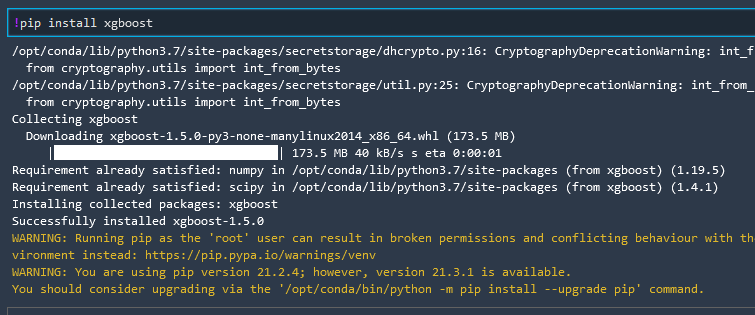
Install XGBoost
!pip install xgboost
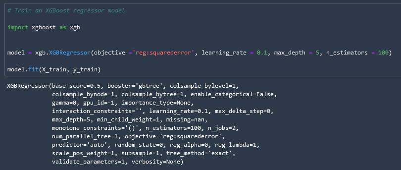
Train XGBoost Regressor Model in Local Mode
Now we can finally train our regressor model
# Train an XGBoost regressor model

import xgboost as xgb


model = xgb.XGBRegressor(objective ='reg:squarederror', learning_rate = 0.1, max_depth = 5, n_estimators = 100)

model.fit(X_train, y_train)
Predict Score with Testing Dataset
# predict the score of the trained model using the testing dataset

result = model.score(X_test, y_test)

print("Accuracy : {}".format(result))
Accuracy : 0.8240983380813032
82% accurracy, great!
Make Predictions on Test Data
# make predictions on the test data

y_predict = model.predict(X_test)
Which gives us an array of 31,618 values in a float32 format array. These are the predicted sales figures output from the X_test data that we fed to our model.

Calculate Metrics
from sklearn.metrics import r2_score, mean_squared_error, mean_absolute_error
from math import sqrt
k = X_test.shape[1]
n = len(X_test)
RMSE = float(format(np.sqrt(mean_squared_error(y_test, y_predict)),'.3f'))
MSE = mean_squared_error(y_test, y_predict)
MAE = mean_absolute_error(y_test, y_predict)
r2 = r2_score(y_test, y_predict)
adj_r2 = 1-(1-r2)*(n-1)/(n-k-1)

print('RMSE =',RMSE, '\nMSE =',MSE, '\nMAE =',MAE, '\nR2 =', r2, '\nAdjusted R2 =', adj_r2)
RMSE = 9779.869
MSE = 95645850.0
MAE = 6435.3916
R2 = 0.8192406043997631
Adjusted R2 = 0.8184539450224686
Automated Amazon Reports
Automatically download Amazon Seller and Advertising reports to a private database. View beautiful, on demand, exportable performance reports.