Intro

In this tutorial we will use multiple linear regression to predict health insurance cost for individuals based on multiple factors (age, gender, BMI, # of children, smoking and geo-location)

Investopedia: Multiple Linear Regression

Import Libraries

import pandas as pd
import numpy as np
import seaborn as sns
import matplotlib.pyplot as plt

Read CSV Data

# read the csv file
insurance_df = pd.read_csv('insurance.csv')

Check for Null Values

# check if there are any Null values
insurance_df.isnull().sum()

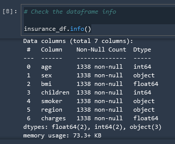
Check DataFrame Info

# Check the dataframe info

insurance_df.info()

Grouping Data

We can group our data with the .groupby() function

# Grouping by region to see any relationship between region and charges
# Seems like south east region has the highest charges and body mass index
df_region = insurance_df.groupby(by='region').mean()
df_region

List Unique Values

It’s actually an array of unique values but…

# Check unique values in the 'sex' column
insurance_df['sex'].unique()

Convert Strings To Numbers

Convert Categorical Variables (boolean) to numerical

We must convert all string based data to numerical data or else we will encounter an error later when we convert everything to float32 format

pandas: .apply()

towardsdatascience.com: apply and lambda usage in pandas

# convert categorical variable to numerical

insurance_df['sex'] = insurance_df['sex'].apply(lambda x: 0 if x == 'female' else 1)

Dummies

Convert all of our string options into a matrix of numerical indicator variables

pandas.get_dummies()

region_dummies = pd.get_dummies(insurance_df['region'], drop_first = True)

Replace Region Column w/ Region Dummies

Now that we have turned our region string column into a matrix of booleans we need to concat the matrix onto the end of the datafield and then remove the region column

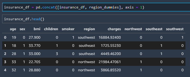
Concat Dummies

insurance_df = pd.concat([insurance_df, region_dummies], axis = 1)

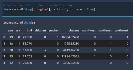
Delete Column (Drop Column)

Rows and Columns can be deleted with the .drop() method.

pandas.drop()

# Let's drop the original 'region' column
insurance_df.drop(['region'], axis = 1, inplace = True)

Visualize The Dataset

Now that we have normalized our data, let’s create a series of histograms for each parameter.

insurance_df[['age', 'sex', 'bmi', 'children', 'smoker', 'charges']].hist(bins = 30, figsize = (20,20), color = 'r')

Regression Line Without Machine Learning

We now have our data shaped into a format that we can use Seaborn to create a regression line without any machine learning. Let’s go ahead and do that.

Here is the linear regression for Age

sns.regplot(x = 'age', y = 'charges', data = insurance_df)
plt.show()

Here is the linear regression for BMI

sns.regplot(x = 'bmi', y = 'charges', data = insurance_df)
plt.show()

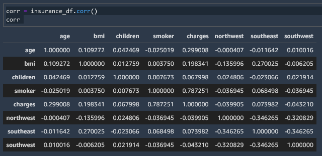
Correlation Matrix Heatmap

We can create a correlation matrix and then convert that to a heatmap to read it more easily

corr = insurance_df.corr()
corr

# resize heatmap so it is legible
plt.figure(figsize = (10,10))
sns.heatmap(corr, annot = True)

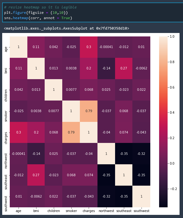
And with this correlation matrix heatmap we can see that the factor with the most correlation to insurance cost is whether or not a person is a smoker.

Create Training and Testing Dataset

Separate Independent and Dependent Variables

Now let’s shape our data into training and testing data sets. Let’s start by separating our independent variables from our dependent variables.

X = insurance_df.drop(columns =['charges'])
y = insurance_df['charges']

And then we can review our new variables

Convert to float32 format

The documentation states that we must convert all numbers to float32 format for regression analysis so lets do that.

X = np.array(X).astype('float32')
y = np.array(y).astype('float32')

After we have converted to float32 let us reshape y so that it has a column

Split Into Train and Test Data

from sklearn.model_selection import train_test_split

X_train, X_test, y_train, y_test = train_test_split( X, y, test_size=0.2, random_state=42)

The random_state here controls the shuffling applied to the data before applying the split. Pass an int for reproducible output across multiple function calls.

📘 sklearn: train_test_split

Scale the Data

In short, the reason why we must scale our data is so that all our features are roughly using the same scale. If a feature has a variance that is orders of magnitude larger that others, it might dominate the objective function and make the estimator unable to learn from other features correctly as expected.

This is not necessary for single feature linear regression because there is only one feature. However this IS required for multiple linear regression.

Data that has been scaled is referred to as normalized data

📘 sklearn: StandardScaler

#scaling the data before feeding the model
from sklearn.preprocessing import StandardScaler, MinMaxScaler

scaler_x = StandardScaler()
X_train = scaler_x.fit_transform(X_train)
X_test = scaler_x.transform(X_test)

scaler_y = StandardScaler()
y_train = scaler_y.fit_transform(y_train)
y_test = scaler_y.transform(y_test)

Train and Test Linear Regression Model in SK-Learn

Note that we are not using SageMaker Algorithms yet. This is a standard SK-Learn model.

# using linear regression model
from sklearn.linear_model import LinearRegression
from sklearn.metrics import mean_squared_error, accuracy_score

regresssion_model_sklearn = LinearRegression()
regresssion_model_sklearn.fit(X_train, y_train)

In the highlighted line we have fit the line

regression_model_sklearn now contains the trained parameters

LinearRegression(copy_X=True, fit_intercept=True, n_jobs=None, normalize=False)

Test Accuracy

Now we can get an accuracy score

regresssion_model_sklearn_accuracy = regresssion_model_sklearn.score(X_test, y_test)
regresssion_model_sklearn_accuracy

0.7835929775784993

So we have achieved about 78% accuracy.

Use Test Data to predict y

Now we can feed in our X_test data that we set aside earlier to get an array of y predictions.

y_predict = regresssion_model_sklearn.predict(X_test)
y_predict

And we can see that we get an array back, however all these numbers look a little small for insurance costs don’t they? Well remember that earlier we normalized this data by scaling it down.

Scale Data Back Up (inverse transform)

And we can see that when we use the inverse transform method of our scaler we get numbers in the range of what we would expect.

y_predict_orig = scaler_y.inverse_transform(y_predict)

y_predict_orig

Calculating the Metrics

We can now calculate some of the metrics that we covered in Ncoughlin: Regression Metrics and KPI’s

from sklearn.metrics import r2_score, mean_squared_error, mean_absolute_error
from math import sqrt

RMSE = float(format(np.sqrt(mean_squared_error(y_test_orig, y_predict_orig)),'.3f'))
MSE = mean_squared_error(y_test_orig, y_predict_orig)
MAE = mean_absolute_error(y_test_orig, y_predict_orig)
r2 = r2_score(y_test_orig, y_predict_orig)
adj_r2 = 1-(1-r2)*(n-1)/(n-k-1)