AWS SageMaker Tutorial: Part 2
Resources
📘 SageMaker Documentation: Linear Learner Algorithm
Intro
In the SageMaker Tutorial Part 1 we learned how to launch SageMaker Studio, import files, launch notebooks, install dependencies and external libraries and start manipulating data using python and several popular libraries. We shaped our basic dataset into training and testing sets and created a linear regression model using 3rd party libraries.
Here in Part 2 we are going to learn how to use the SageMaker built in algorithms and build a machine learning model the "SageMaker way".
Import Libraries
Let's start by importing the SageMaker libraries that we need and defining our S3 bucket that we will be using.
# Boto3 is the Amazon Web Services (AWS) Software Development Kit (SDK) for Python
# Boto3 allows Python developer to write software that makes use of services like Amazon S3 and Amazon EC2

import sagemaker
import boto3
from sagemaker import Session

# Let's create a Sagemaker session
sagemaker_session = sagemaker.Session()

# Let's define the S3 bucket and prefix that we want to use in this session
bucket = 'tutorial-sagemaker-employee-linear-learner' # bucket named 'sagemaker-practical' was created beforehand
prefix = 'linear_learner' # prefix is the subfolder within the bucket.

# Let's get the execution role for the notebook instance.
# This is the IAM role that you created when you created your notebook instance. You pass the role to the training job.
# Note that AWS Identity and Access Management (IAM) role that Amazon SageMaker can assume to perform tasks on your behalf (for example, reading training results, called model artifacts, from the S3 bucket and writing training results to Amazon S3).
role = sagemaker.get_execution_role()
print(role)
down at the bottom there we can see that we also looked up the IAM role that is associated with this SageMaker instance. This role will need permission to access your S3 bucket so we can read from it and then write artifacts to it later.
Shape Training Data
Let's quickly review the shape of our data and then shape our y_train set into a vector. It appears that the target label must always be a vector...

Convert Data to RecordIO format
If we review the SageMaker Linear Learner documentation we know that our data is required to be in RecordIO format. So let us convert our training data into RecordIO.
import io # The io module allows for dealing with various types of I/O (text I/O, binary I/O and raw I/O).
import numpy as np
import sagemaker.amazon.common as smac # sagemaker common libary

# Code below converts the data in numpy array format to RecordIO format
# This is the format required by Sagemaker Linear Learner

buf = io.BytesIO() # create an in-memory byte array (buf is a buffer I will be writing to)
smac.write_numpy_to_dense_tensor(buf, X_train, y_train)
buf.seek(0)
# When you write to in-memory byte arrays, it increments 1 every time you write to it
# Let's reset that back to zero
At this point our training data is contained in the buf variable.
Upload training data to S3 Bucket
Remember that our SageMaker Data is always pulled from S3, and artifacts are returned to S3. Therefore we need to send our training data to our S3 Bucket.
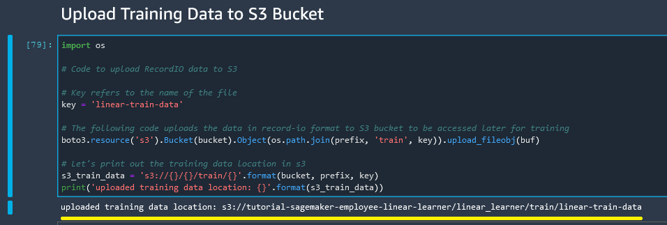
import os

# Code to upload RecordIO data to S3

# Key refers to the name of the file
key = 'linear-train-data'

# The following code uploads the data in record-io format to S3 bucket to be accessed later for training
boto3.resource('s3').Bucket(bucket).Object(os.path.join(prefix, 'train', key)).upload_fileobj(buf)

# Let's print out the training data location in s3
s3_train_data = 's3://{}/{}/train/{}'.format(bucket, prefix, key)
print('uploaded training data location: {}'.format(s3_train_data))
And our training data location appears to be correct.
So at this point we have converted our training data into a buffer and uploaded to an S3 bucket and set variable s3_train_data to our bucket location.
Repeat Process for Test Data
Next we repeat that same process for our test data so that it is also available to SageMaker.
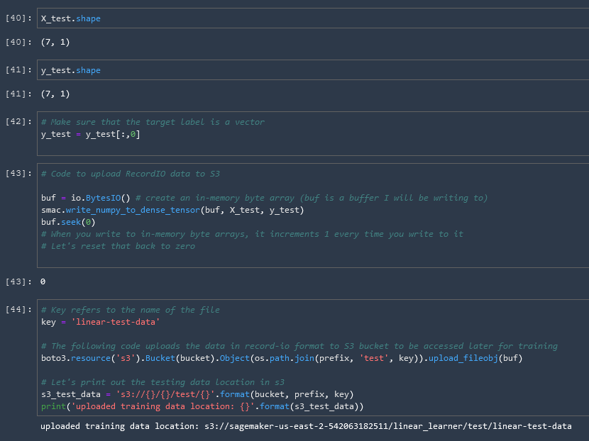
Create Output Placeholder
Next let us create a placeholder in our S3 bucket to hold the output of the model.
# create an output placeholder in S3 bucket to store the linear learner output

output_location = 's3://{}/{}/output'.format(bucket, prefix)
print('Training artifacts will be uploaded to: {}'.format(output_location))

And that concludes the configuration of our S3 Bucket.
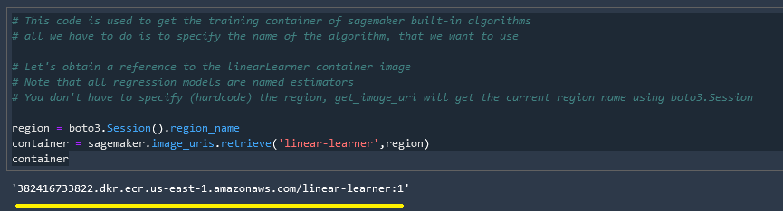
Get Algorithm Container
Sagemaker Algorithms are Dockerized, and we need to tell our model where that docker image (container) exists. To find the location we use the sagemaker.image_uris.retrieve() function, with the arguments being which model we would like to retrieve and our region. More about this in the documentation.
# This code is used to get the training container of sagemaker built-in algorithms
# all we have to do is to specify the name of the algorithm, that we want to use

# Let's obtain a reference to the linearLearner container image
# Note that all regression models are named estimators
# You don't have to specify (hardcode) the region, get_image_uri will get the current region name using boto3.Session

region = boto3.Session().region_name
container = sagemaker.image_uris.retrieve('linear-learner',region)
container
Select & Run Training Algorithm
Now we take all of pieces that we have prepared beforehand, select our algorithm options and train the model!
# We have to pass in the container, the type of instance that we would like to use for training
# output path and sagemaker session into the Estimator.
# We can also specify how many instances we would like to use for training
# sagemaker_session = sagemaker.Session()

linear = sagemaker.estimator.Estimator(container,
                                       role,
                                       instance_count = 1,
                                       instance_type = 'ml.c4.xlarge',
                                       output_path = output_location,
                                       sagemaker_session = sagemaker_session)


# We can tune parameters like the number of features that we are passing in, type of predictor like 'regressor' or 'classifier', mini batch size, epochs
# Train 32 different versions of the model and will get the best out of them (built-in parameters optimization!)

linear.set_hyperparameters(feature_dim = 1,
                           predictor_type = 'regressor',
                           mini_batch_size = 5,
                           epochs = 5,
                           num_models = 32,
                           loss = 'absolute_loss')

# Now we are ready to pass in the training data from S3 to train the linear learner model

linear.fit({'train': s3_train_data})

# Let's see the progress using cloudwatch logs
And we can see that our model is successfully being trained.

Reduce Billable Seconds w/ Spot Instances
One of the very useful parameters available to us is the use of spot instances to reduce billable seconds. This is essentially just spare EC2 instances that are sitting around without any jobs running on them, we can piggyback on them to execute our tests for a reduced cost.
linear = sagemaker.estimator.Estimator(container,
                                       role,
                                       instance_count = 1,
                                       instance_type = 'ml.c4.xlarge',
                                       output_path = output_location,
                                       sagemaker_session = sagemaker_session,
                                       use_spot_instances = True,
                                       max_run = 300,
                                       max_wait = 600
                                      )
Adding these options reduced the billable seconds on this model from 44 => 26, but increased the total execution time from 44 => 79. So depending on how much of a hurry you are in this could save you a lot of money!
Deploy Model
💵 Cost Warning: Note that deploying the model spins up an EC2 instance which will run until the model is shut down, which of course costs money. So if you are not actively using a model, shut it down or be prepared to pay for it!
# Deploying the model to perform inference

linear_regressor = linear.deploy(initial_instance_count = 1,
                                          instance_type = 'ml.m4.xlarge')
Content Type & Serializers
In order to make inferences on the model we need to pass in the data in a 'text/csv' format. To aid in that we define for our model which methods of serialization and deserialization we should be using.
from sagemaker.serializers import CSVSerializer
from sagemaker.deserializers import JSONDeserializer

# Content type overrides the data that will be passed to the deployed model, since the deployed model expects data in text/csv format.

# Serializer accepts a single argument, the input data, and returns a sequence of bytes in the specified content type

# Deserializer accepts two arguments, the result data and the response content type, and return a sequence of bytes in the specified content type.

linear_regressor.serializer = CSVSerializer()
linear_regressor.deserializer = JSONDeserializer()
Making a prediction with the model
We are ready to make a prediction using our model. Let's pass in our test data and see what we get.
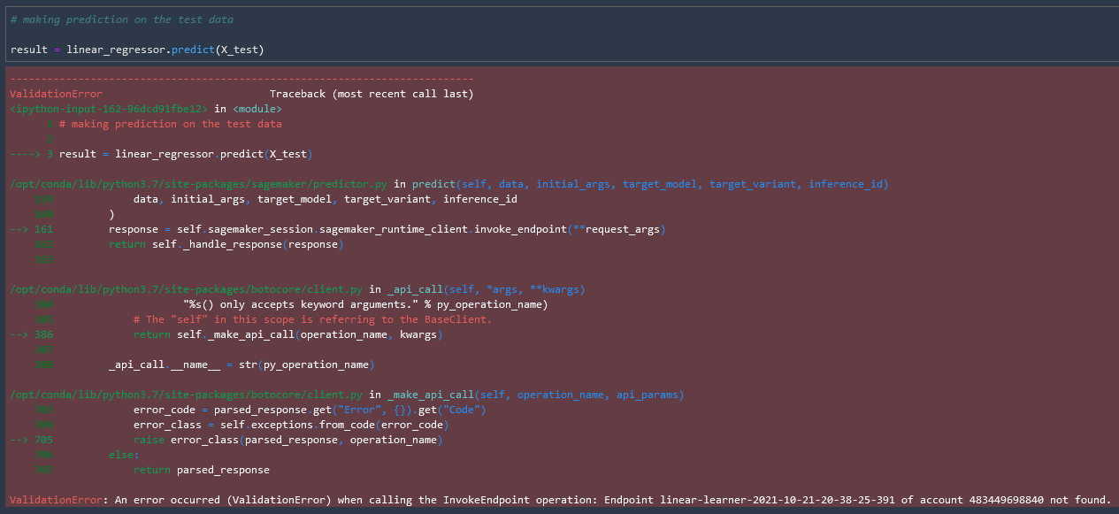
# making prediction on the test data

result = linear_regressor.predict(X_test)
result # results are in Json format
{
  "predictions": [
    { "score": 87283.6953125 },
    { "score": 84392.9921875 },
    { "score": 20797.421875 },
    { "score": 22724.5625 },
    { "score": 39105.2421875 },
    { "score": 76684.4375 },
    { "score": 94992.2578125 }
  ]
}
And we can see our results in JSON format. Le'ts reformat that into an array using the numpy array function
.array()
# Since the result is in json format, we access the scores by iterating through the scores in the predictions

predictions = np.array([r['score'] for r in result['predictions']])
predictions

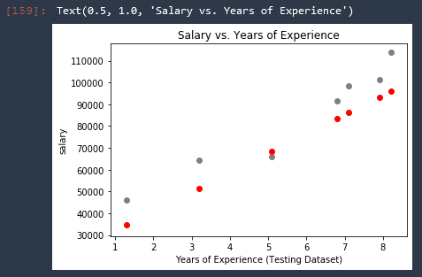
Visualize Results
Lastly we can plot the results of our predictions vs our test data.
# VISUALIZE TEST SET RESULTS
plt.scatter(X_test, y_test, color = 'gray')
plt.scatter(X_test, predictions, color = 'red')
plt.xlabel('Years of Experience (Testing Dataset)')
plt.ylabel('salary')
plt.title('Salary vs. Years of Experience')
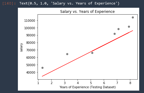
The predicted salaries are of course all on the same line, therefore we can just replace that with a line!
# VISUALIZE TEST SET RESULTS
plt.scatter(X_test, y_test, color = 'gray')
plt.plot(X_test, predictions, color = 'red') # highlight-line
plt.xlabel('Years of Experience (Testing Dataset)')
plt.ylabel('salary')
plt.title('Salary vs. Years of Experience')
Delete End-Point
Now that we are finished with this model, let us go ahead and delete the endpoint (shut down the EC2 instance) so that we don't have to keep paying for it to run.
# Delete the end-point

linear_regressor.delete_endpoint()
Now if we try to run the model again we get an error "Endpoint not found". Perfect!
Automated Amazon Reports
Automatically download Amazon Seller and Advertising reports to a private database. View beautiful, on demand, exportable performance reports.